MS: ✓
BS: ✗
2-Dimensional Spectrum Analysis
For more information, see:
An acceptable method for the approzimation for most systems is the model for a mixture of individual non-interacting solutes as described by the Lamm equation.1 The Lamm Equation2 descibes the sedimentation and diffusion transport of a single ideal solute in an AUC cell. Therefore, for a mixture of non-interacting solutes, the total concentration \(C_{T}\) of all solutes \(n\) can be represented by a sum of Lamm equation solutions \(L\):
Finding the correct values of \(c_{i}\), \(s_{i}\), and \(D_{i}\) is the challenge when fitting experimental velocity data, and require an optimziation approach that can deal with the non-linearity.
One way of doing this is to use iterative fitting methods using non-linear squares optimization.34[^Schuck1998] But there are drawbacks:
-
the correct model must be selected and verified by user leading to bias in analysis, and;
-
the non-linear least squares tends to break down for systems containing three of more components. This is due to the complexity of the error surface, where simply gradient descent methods fail to navigate the complex, multi-dimensional error surfaces, tending to be traped by local minima, never converging to the global optima. It can also be due to the presence of multiple minima with nearly identical residuals, or the failure to consider additional signals from the inadequacy of the selected models.
The C(s) method56 was developed to address these drawbacks by implementing a system linearization avoiding multi-dimensional searchs by iterative methods. In an extention of c(s) method, a regularized searchover a course grid of both \(s\) and \(f/f_{0}\) was added. The idea behind this linearization method is as follows:
-
the sedimentation ocefficient range is assumed to represened by the solutes in the experiment, divided into equidistant partitions.
-
the diffusion coefficent is treated as a constant and is parameterized with the sedimentation coefficient, \(s\), and frictional ratio, \(k = f/f_{0}\):
- The constant \(k = f/f_{0}\) is held constant throughout our \(C_{T}\) equation, so that only coefficeint \(c_{i}\) need to be determined, while assuming that the coefficients are only greater than or equal to zero.
Therefore, for the C(s) method, a single-dimensional non-linear search over \(k\) is added to identify an approximate weight average \(k\) for \(\textbf{all}\) solutes present. This raises several concerns. First, by treating \(k\) to be constant, generality is sacrified. It will only be sufficient for single components, or if all species in a mixture are spherical and the frictinoal ratio is equal to 1. In heterogenous mixtures, when this average frictional ratio value is used to transfform the \(s\)-value distrubtion into a molecular weight distribution, there will be an overestimatization of the molecular weight of the most globular component, and an underestimization of the least globular components molecular weight.
To address this issue, Brookes and Demeler, amoung others, have explored stochastic search algorithms, with evidencing showing that it is possible to resolve more than two comonents in a mixture with the same level of detail as direct boundary fitting methods. However, these methods require comparatively higher computational efforts, and are impractical for implementing to workstations.
Overall, the C(\(s, f/f_{0}\) method suffers from:
-
a lack of resolution;
-
large memory needs;
-
producing unnecessarily broad molecular weight distributions, and;6
-
introducing false positives caused by noise in the data and by failing to consider the entire parameter space in each minimization step.
The 2DSA method is a model-independent approach for fitting sedimentation velocity data which permits simultaneous determination of shape and molecular distributions for mono- and polydisperse solutions of macromolecules. 2DSA is based on fine grained 2-D grid searches over sedimentation coefficients and frictional ratios. The grid is a linear combination of whole boundary models represented by finite element solutions of the Lamm equation. Grid points correspond to the sedimentation and diffusion coefficients present in the Lamm equation. This approach allows for heterogeneity in the frictional domain. This allows for a more faithful description of the experimental data for cases where frictional ratios are not identical for all components. As a result of allowing frictional heterogeneity, the 2DSA method allows for a more reliable molecular weight distributions.
Overall, the 2DSA method allows for:
-
globablly fitting multi-speed experiments;
-
the elimination of time- and radially- invarient noise;
-
use on a single work station in a serial implementation or in a parallel computing environment for improved computational seed;
-
superiour accuracy and lower variance fits to experimentat data;
-
identifying modes of aggregation and slow polymerization, and;
-
characterizing confidence limits for determined solutes using Monte Carlo approaches.
The examples presented below will demonstrate that, for non-interacting systems, the 2DSA approach is general and model-independent, and does not depend on prior knowledge of the underlying model. For mixtures of rapidly equilibibrating solutes, this approach provides approximations for solutes distributions (although interaction coefficients like equilibiurm and rate constants cannot be obtained). This method also simultaneoulsy resolves heterogeneity in shape and in molecular weight or sedimentation coefficients at a very high resolution, while producing well defined and narrow solute boundaries.
Description of Method
The 2DSA method is built on the approach of modeling experimental seimentation data by building a two-dimensional grid of frictional ratios and sedimentation coefficients. Using the van Holde-Weischet method or the \(d\)C\(/dt\) method, one can obtain a knowledge of the fitting limits for \(s\) and \(f/f_{0}\), which is the only user input required by the 2DSA. the \(d\)C\(/dt\) mwrhod is preferred for initialization when there is significant time-invariant noise, as it is superiour in its handling capabilities.
To parameterize the diffusion coefficient, it is convinient to use the frictional ratio. Recall the diffusion equation presented above. Using that equation, a unique value for \(s\) and \(D\) can be defined at each grid point. This can also be used to simulate a velocity exeriment for a species with those specific parameters. To simulate all Lamm equation models, you can use the adaptive space-time finite element solution,11 and built the sum:
where \(s_{i}\) is the sedimentaiton coefficient at position \(i\), the fricitonal ratio at \(j\) is \(k_{j}\), \(m\) is the number of grid points in the sedimentation domain, and \(n\) is the number of grid points in the fricitonal ratio domain. The parital concentration of the simulated solutes at grid points \((i,j)\) is then \(c_{i,j}\).
The minimization problem can be states as the task of finding the minimum for the \(l^{2}\)-norm:
where \(E_{r,t}\) referes to teh experimentally determined data points for \(h\) radial points \(r\) and \(l\) time scans \(t\). The minimization problem is solved using the NNLS algorithm,9 while simultaneoulsy algebraically accounting for the time- and radially- invariant noise contributions in the experimental data.[^SchuckDemeler1999]
The linear optimization, in matrix form, is:
where \(\bf{A}\) is the matrix of finite element solutions, \(x\) is the solution vector containng all coefficients \(c_{i,j}\), and \(\bf{b}\) is the vector of experimental data.
MULTI-STAGE REFINEMENT: Lorem ipsum lorem ipsum lorem ipsum lorem ipsum lorem ipsum lorem ipsum.
SIMULATION OF GRID ELEMENTS: The ASTFEM solution10 is used to simulate the Lamm equation solutions for each grid point. You can take advantage of the invariance:
where \(a\) is a multiplier that cover the entire desired range of \(s\) and \(D\) values, to reduce computational effort.
ITERATIVE REFINEMENT: Solving the iterative problem involving mutiple low resolution sub-gribs can be empirically shown to be equivalent to solving a high resolution grid covering the same grid points, if the following operations are performed: the non-zero grid points evaluated at the final state are joined with each original grid and processed. The analysis is repeated until convergence is obtained such that an sparse parameter distribution with discrete solutes is identified from the experimental data.
Note that this method will not converge to exactly the same solution when time- or radially- invariant noise corrections are performed simulataneously, but these difference are negliable.
Example 1
2DSA-Monte Carlo analysis of a 2-component system with heterogeneity in mass and shape
In order to illustrate the ability of the 2DSA method to resolve a system that is heterogeneous in molecular weight and shape, the following system was used. It consisted of:
-
a globular protein (heen egg lyzosyme), and;
-
an elongated molecule (208 bp linear fragment of double-stranded DNA).
The lyzosyme has a partial specific volume of 0.724 ccm/g and the DNA has a partial specific volume of 0.55 ccm/g.
These molecules were mixed in approximately equally absorbing amounts in 200 mM NaCL and 25 mM TRIS buffer at pH 8.0. The mixture was then run at 42,000 rpm in the standard 2 channel centerpeices, with velocity data collected for 3 hours at 260 nm.
Time invariant noise was subtracted so that only stochatic noise would remain in the data.7 This data was then fitting with the 2DSA method using 50 Monte Carlo iterations, using the iterative refinement method with a maximum of 5 iterations.8
Figure: 2DSA Monte Carlo Analysis of Velocity Data
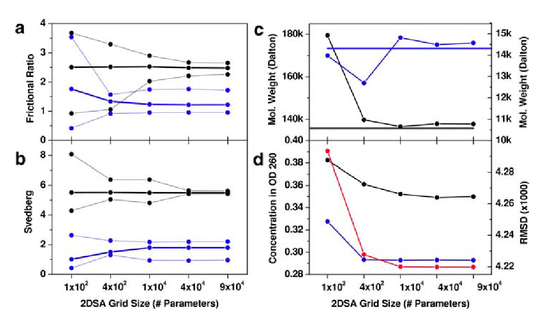
2DSA Monte Carlo analysis of velocity data from a mixture of a 208 bp DNA fragment (black lines) and hen egg lysozyme (blue lines). Heavy lines indicate the mean, thin lines represent 95% confidence intervals for the parameter.
The results for several parameters from multiple grid resolutions are compared.
\(\textbf{a}\) frictional ratio;
\(\textbf{b}\) sedimentation coefficient (corrected to standard conditions);
\(\textbf{c}\) molecular weight, horizontal lines indicate theoretical molecular weight based on sequence;
\(\textbf{d}\) partial concentration and the residual mean square deviation of the fit (red line).
Reliable results are obtained after a minimum of 10,000 iterations; higher resolutions do not improve the results significantly.
The following observations were made:
-
The 2DSA is a very robust method. Additonal degenergy was introduced when the resolution of the grid was increased but it did not degrade the solutions reliability.
-
The method faithfully reproduces known molecular weights with great precision and accuracy when adjusted for the appropraite partial specific volumes.
-
There is additional benefit derived when using iterative refinements.
Figure 1: Pseudo-3D plots for 2DSA Monte Carlo Results
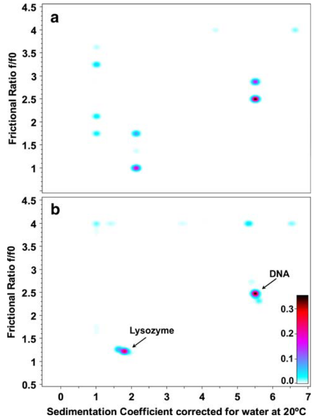
Pseudo-3D plots for solute distributions from the 2DSA Monte Carlo results for the highest and lowest grid resolutions.
\(\textbf{a}\) grid resolution for 100 solutes;
\(\textbf{b}\) grid resolution for 90,000 solutes.
At the low resolution, the composition is porrly defined and the solute peaks are split. At higher resolutions, both species are well defined into narrow regions. Noise contributions are well seperated and idenifiable by the upper frictional ratio fitting limit (\(k=f/f_{0}\)=4). The color scale represents the signal of each species in optical density units.
Example 2
Multi-speed 2DSA-Monte Carlo analysis of a simulated 5-component system with heterogeneity in mass and shape
The simulated system consisted of equal concentrations of a linearly elongated aggregate and five non-interacting components:
-
monomer (25 kDa, \(f/f_{0}\)=1.2);
-
dimer (50 kDa, \(f/f_{0}\)=1.4);
-
tetramer (100 kDa, \(f/f_{0}\)=1.6);
-
octomer (200 kDa, \(f/f_{0}\)=1.8);
-
hexadecamer (400 kDa, \(f/f_{0}\)=2.0).
Each simulation contained 70 equally spaced scans, resulting in experiment length of ~128 hours at 10 krpm, ~14 hours at 30 krpm, and ~3.5 hours at 60 krpm.
Figure 2: Pseduo-3D plots for 2DSA Monte Carlo Results (Multi-Speed)
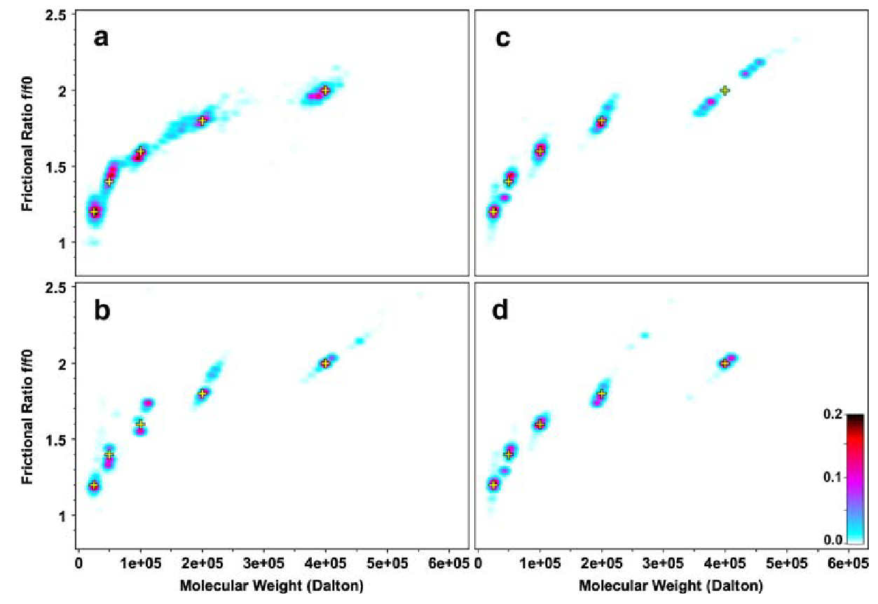
Pesudo-3D plots for Monte Carlo 2DSA analysis resuls for a simulated five-component system.
\(\textbf{a}\) single speed fit (10 krpm), concentional centerpiece;
\(\textbf{b}\) single speed fit (60 krpm), conventional centerpiece;
\(\textbf{c}\) global multi-speed fit (10, 30, 60 krpm), conventional centerpiece;
\(\textbf{d}\) global multi-speed fit (10, 30, 60 krpm), conventional and band-forming Vinograd centerpeice combined.
Yellow crosses indicate the position of known solutes that were simulated for the original data. The color scale represents the signal of each species in optical density units.
From the multi-speed pseudo-3D plots above, the following observations were made:
-
Single speed fits at 10 krpm with the conventional centerpeice shows poorly resolved signal bands.
-
Single speed fits at 60 krpm with the conventional centerpiece shows more precise defintion of the horizonatal domain, but has a poorly defined frictional range.
-
The global multi-speed fit with the conventional centerpiece eliminates the peak splitting of the medium sized species (tetramer, 100 kDa). However the hexadecamer (400 kDa) was poorly defined with peak splitting.
-
The best fit with full peak splitting resolved is found in the global multi-speed fit when combining data from the conventional centerpiece and the band-forming Vinograd centerpiece. Here, all determined signals fit exceptionally well to the starting parameters.
-
Schuck, P. (2003). On the analysis of protein self-association by sedimentation velocity analytical ultracentrifugation. Analytical Biochemistry, 320(1), 104-124. https://doi.org/10.1016/S0003-2697(03)00289-6↩
-
Lamm, O. (1929). Die differentialgleichung der ultrazentrifugierung. Almqvist & Wiksell.↩
-
Todd, G., & Haschemeyer, R. (1981). General solution to the inverse problem of the differential equation of the ultracentrifuge. Proc Natl Acad Sci USA, 78(11), 6739-6743.↩
-
Demeler, B., & Saber, H. (1998). Determination of Molecular Parameters by Fitting Sedimentation Data to Finite-Element Solutions of the Lamm Equation. Biophysical Journal, 74(1), 444-454. https://doi.org/10.1016/S0006-3495(98)77802-6↩
-
Schuck, P. (2000). Size-Distribution Analysis of Macromolecules by Sedimentation Velocity Ultracentrifugation and Lamm Equation Modeling. Biophysical Journal, 78(3), 1606-1619. https://doi.org/10.1016/S0006-3495(00)76713-0↩
-
Brown, P. H., & Schuck, P. (2006). Macromolecular Size-and-Shape Distributions by Sedimentation Velocity Analytical Ultracentrifugation. Biophysical Journal, 90(12), 4651-4661. https://doi.org/10.1529/biophysj.106.081372↩↩
-
Schuck, P., & Demeler, B. (1999). Direct Sedimentation Analysis of Interference Optical Data in Analytical Ultracentrifugation. Biophysical Journal, 76(4), 2288-2296. https://doi.org/10.1016/S0006-3495(99)77384-4↩
-
Demeler, B., & Brookes, E. (2008). Monte Carlo analysis of sedimentation experiments. Colloid and Polymer Science, 286(2), 129-137. https://doi.org/10.1007/s00396-007-1699-4↩
-
Lawson, C., & Hanson, R. (1974). Solving least square problems. Prentice-Hall, Englewood Cliffs.↩
-
Cao, W., & Demeler, B. (2008). Modeling Analytical Ultracentrifugation Experiments with an Adaptive Space-Time Finite Element Solution for Multicomponent Reacting Systems. Biophysical Journal, 95(1), 54-65. https://doi.org/10.1529/biophysj.107.123950↩
-
Cao, W., & Demeler, B. (2005). Modeling Analytical Ultracentrifugation Experiments with an Adaptive Space-Time Finite Element Solution of the Lamm Equation. Biophysical Journal, 89(3), 1589-1602. https://doi.org/10.1529/biophysj.105.061135↩